Analysis of spatially resolved ATAC-seq data
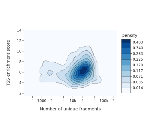
Fastq from the paper “Spatial epigenome–transcriptome co-profiling of mammalian tissues” (Zhang et al, 2023, DOI:10.1038/s41586-023-05795-1) were downloaded (SRA run ID: SRR22565186) and processed using chromap. The resulting fragment file is imported using snapatac2. Here’s just a plot showing the general performance of the spatial ATAC-seq data.
First of all, we import all required libraries.
import numpy as np
import pandas as pd
import matplotlib
import matplotlib.pyplot as plt
from matplotlib.pyplot import *

import anndata as ad
import scanpy as sc
import snapatac2 as snap

import scipy.sparse as ssp
import scipy.stats as sst

import spatialdata_io
import spatialdata_plot
import spatialdata as sd

import squidpy as sq
import schist as scs
import warnings
warnings.filterwarnings('ignore')
#import magic
from tqdm import tqdm

def set_res(high=True):
        dpi=80
        if high:
                dpi=150
        sc.set_figure_params(dpi=dpi, fontsize=6)
        rcParams['axes.grid'] = False

set_res(False)
Parsing of fragment is performed using standard parameters. THe whitelist here is the list of all 2500 barcodes allowed by the DBiT-seq circuit.
adata = snap.pp.import_data('SRR22565186.bed.gz',
                             sorted_by_barcode=False,
                                                         whitelist='whitelist.txt', backend=None,
                                                         chunk_size=20000,
                                                         min_num_fragments=0,
                                                         chrom_sizes=snap.genome.mm10)
snap.pl.frag_size_distr(adata, interactive=False)
snap.metrics.frip(adata, {"peaks_frac": snap.datasets.cre_HEA()})
snap.metrics.tsse(adata, snap.genome.mm10)
snap.pl.tsse(adata, interactive=False, )
We bin genome at 1000 bp, apply some filters and apply snapatac’s fast dimensionality reduction scheme after selecting variable features. We save the .h5ad file that is used to build a spatialdata object
snap.pp.add_tile_matrix(adata, counting_strategy='paired-insertion', bin_size=1000)
adata.obs['log_fragment'] = np.log10(adata.obs['n_fragment'])
cells = adata.obs.query('n_fragment >= 5000 and tsse >= 3 and n_fragment <=100000').index
adata = adata[cells].copy()
#select the top 50k regions
snap.pp.select_features(adata,
                    filter_upper_quantile=0.,
                    n_features=50000,
                    max_iter=1, blacklist='mm10-blacklist.v2.bed.gz')
snap.tl.spectral(adata)
adata.write("analysis/atac_raw.h5ad")
Here the anndata is imported using the DBiT-seq plugin for spatialdata. Note that we had to rotate the original image from the paper 90 degrees CCW, as the current version of the plugin orders the barcodes differently from what is displayed in the original paper.
spdata = spatialdata_io.readers.dbit.dbit(path='analysis',
                                        anndata_path='analysis/atac_raw.h5ad',
                                        barcode_position='barcodes.txt',
                                        image_path='ME13_50um_spatial/tissue_hires_image.png',
                                        dataset_id='ME13_50um_spatial'
                             )
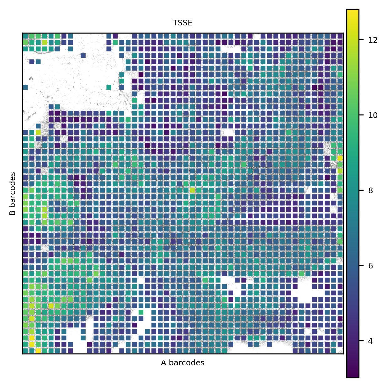
The TSS enrichment is visualized in its spatial context. The eye and the forebrain regions have the highest TSSE values.
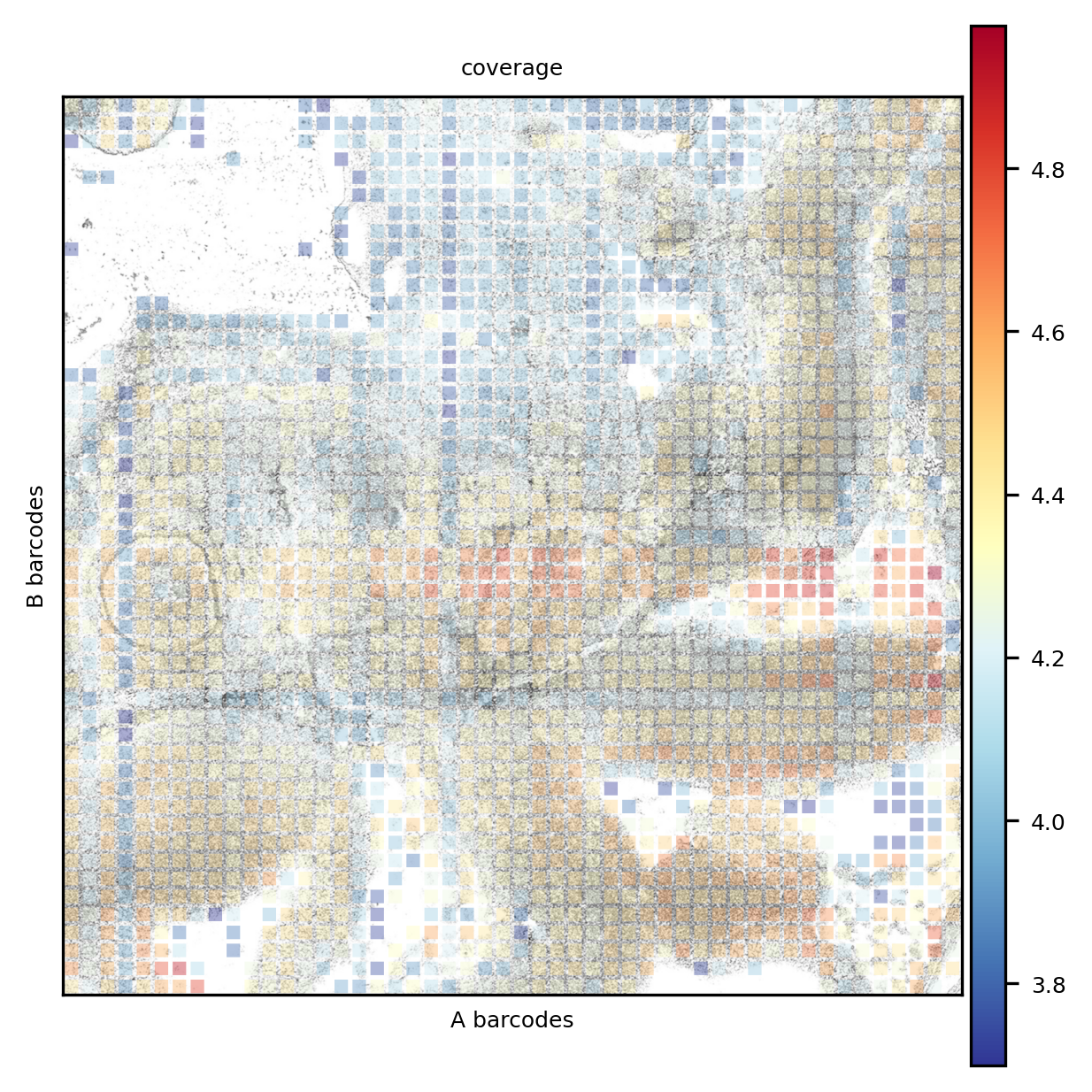
The coverage is unevenly distributed. We here notice an issue common in DBiT-seq, that is some channels _stripe_ the tissue because of differences in the flows.
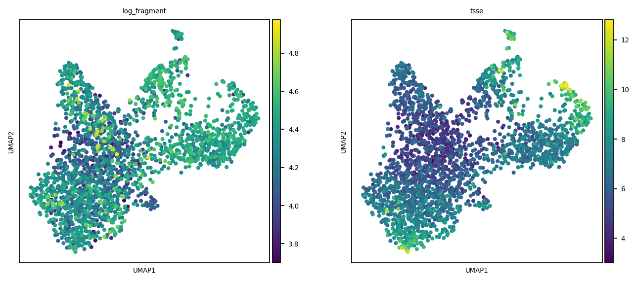
We here create the kNN graph, according to the spectral reduction performed above. A UMAP plot is also presented (not that we are going to use it, anyway).
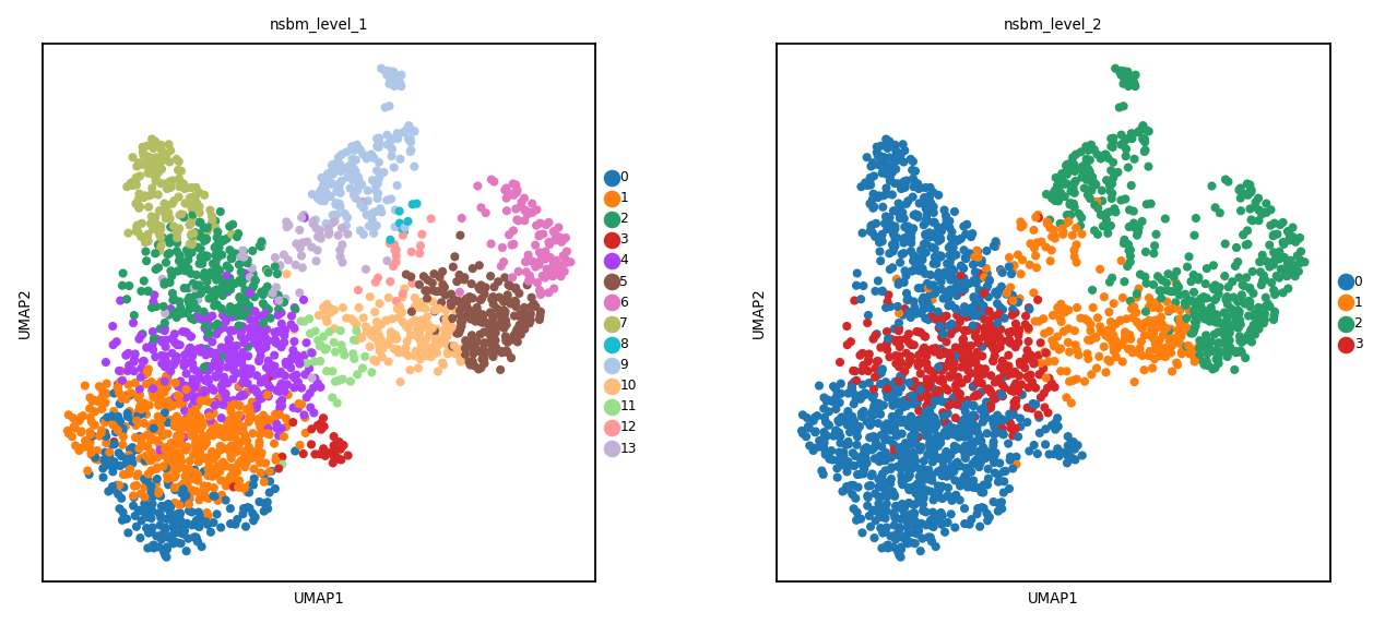
Here a simple hierarchical model is performed using schist on the kNN graph above. The clusters at level 1 and 2 are shown in UMAP.
basis='spectral'
sc.pp.neighbors(spdata.table, key_added=f'{basis}_neighbors', use_rep=f'X_{basis}')
sc.settings.verbosity=2
scs.inference.fit_model(spdata.table, neighbors_key=f'{basis}_neighbors')
sc.settings.verbosity=0
minimizing the nested Stochastic Block Model
        minimization step done (0:01:28)
        consensus step done (0:01:46)
    done (0:01:46)
    finished (0:01:46)
sc.pl.umap(spdata.table, color=['nsbm_level_1', 'nsbm_level_2'])
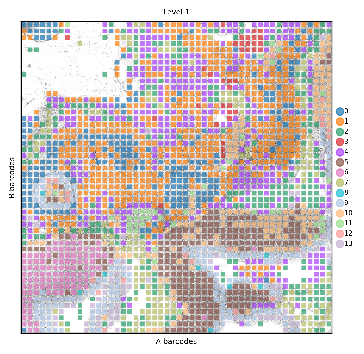
Finally we can check how clusters distribute in their spatial context. At level 1 we can distinguish certain clusters that belong to the neual tissues.
set_res(True)
spdata.pl.render_images().pl.render_shapes(color='nsbm_level_1', fill_alpha=.7).pl.show(title='Level 1', colorbar=True)
xticks([])
yticks([])
plt.xlabel('A barcodes')
plt.ylabel('B barcodes')
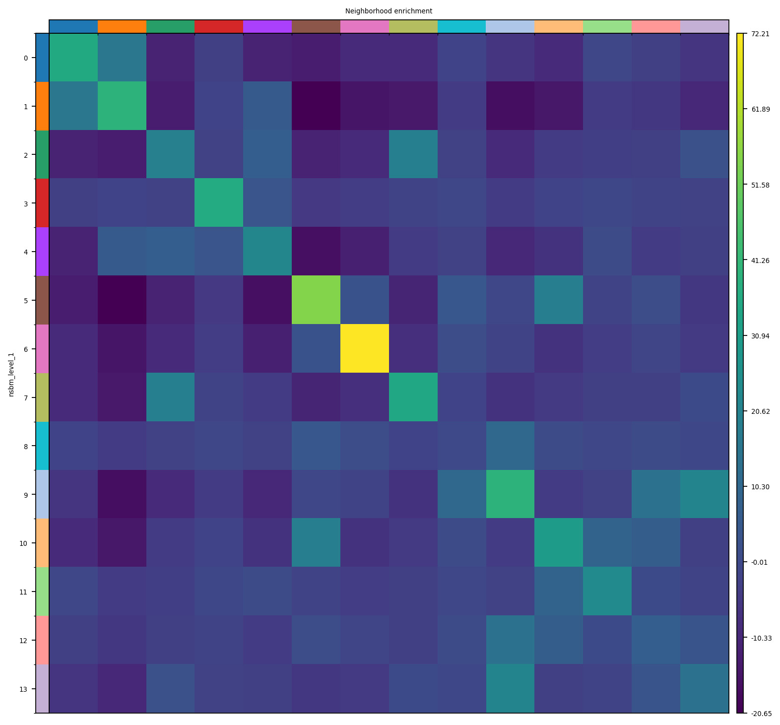
The neural clusters are also the ones with highest self-enrichment in their neighborhood.
sq.gr.spatial_neighbors(spdata.table, n_neighs=8, coord_type='grid')
sq.gr.nhood_enrichment(spdata.table, cluster_key="nsbm_level_1")
set_res(False)
sq.pl.nhood_enrichment(spdata.table, cluster_key="nsbm_level_1")
Can we perform better than this? One idea would be to integrate the spatial information into the model. Spatial data, especially for grid-like data as in DBiT-seq, do not have a community structure, yet they can be used to enforce local communities. schist does not yet support spatial graphs with a specific function, however we can create an object with a spatial graph (copying the original) and apply the multimodal nested solution, specifying the two graphs needed.
_tmp = spdata.table.copy()

sc.settings.verbosity=2
scs.inference.fit_model_multi([spdata.table, _tmp],
                              key_added='spt',
                              neighbors_key=['spectral_neighbors', 'spatial_neighbors'])
sc.settings.verbosity=0
minimizing the nested Stochastic Block Model
getting adjacency for data 0 (0:00:00)
getting adjacency for data 1 (0:00:00)
        minimization step done (0:05:39)
        consensus step done (0:05:50)
    done (0:05:50)
    finished (0:05:50)
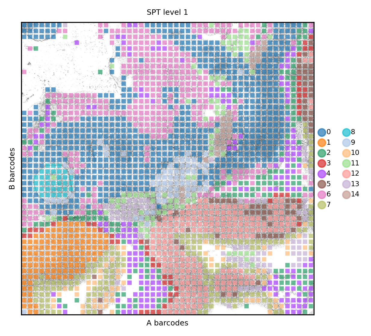
The process takes more time than above, but the results are clearly matching the anatomycal structures. We now see clusters 9 and 13 marking two structures that were not visibile in the original publication, if not with RNA-seq
set_res(True)
spdata.pl.render_images().pl.render_shapes(color='spt_level_1', fill_alpha=.7).pl.show(title='SPT level 1', colorbar=True)
xticks([])
yticks([])
plt.xlabel('A barcodes')
plt.ylabel('B barcodes')
We save the results for later analysis
spdata.write('analysis/SRR22565186.zarr')