Analysis of large datasets
It is stated in the original paper
(and also raised by users) that schist may be slow, especially for
large datasets. While the underlying library is computationally
efficient, the MCMC problem may be difficult to minimize and scales with
the square of the number of the edges. In lay terms, this means that the
number of cells and the number of neighbors used to build the kNN graph
will, in turn, influence the speed of the procedure. Moreover, it is
difficult to predict the actual execution time due to the specific
nature of the data. In other words, there are datasets in which the
algorithms converges pretty fast because the community structure is
“easy to find”.
While we are working on an appropriate solution, which may require complete rewriting of the library, there is one workaround that works in most cases, although the solution is not optimal. The solution goes through the analysis of multiple subsamples of the data. Since the MCMC does not scale linearly with the data size, the time required to analyze subsample is possibly smaller than the time required to analyze the full data. Of course, there’s a huge drawback, that is the final solution won’t ever have the same resolution and will find larger communities.
The following tutorial goes through the analysis of the HCA Lung datasets, downloaded from the cellxgene data portal, which includes more than 2 millions cells.
import scanpy as sc
import schist as scs
import graph_tool.all as gt
import sklearn.neighbors as skn
import sklearn.metrics as skmt
import numpy as np
import matplotlib as mpl
import matplotlib.pyplot as plt
from matplotlib.pyplot import *
from pynndescent import NNDescent
import anndata as ad
import scipy.sparse as ssp
import pandas as pd
from tqdm import tqdm
import warnings
warnings.filterwarnings('ignore')
%matplotlib inline
sc.set_figure_params()
rcParams['axes.grid'] = False
The dataset is rather huge (20 Gb), we will perform operations without loading it into memory. Whenever we will need to modify its attributes, we will create a lightweight copy, including only the relevant information.
adata = sc.read("local.h5ad", backed='r')
print(adata.shape)
(2282447, 56295)
The Planted Partition Model
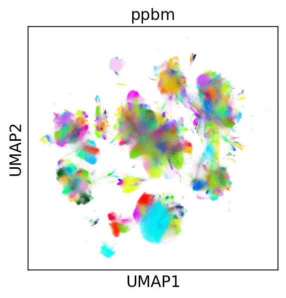
Before going with subsampling, we show the results of a
ppbm calculated on this dataset using a single iteration,
in place of the 100 typically performed with schist. It took
approximately 13 hours to converge, which is long but possibly
tractable, if you consider we are dealing with 2M cells
import pickle
full_ppbm_state = pickle.load(open("HCA_full_ppbm.pickle", "rb"))
print(full_ppbm_state)
<PPBlockState object with 256 blocks, for graph <GraphView object, undirected, with 2282447 vertices and 51427121 edges, at 0x7f6f027728f0>
Unfortunately, the model contains more than 100 blocks (256), so it
cannot be visualized properly using scanpy plotting facilities.
Hence, we create the appropriate number of colors choosing from a
continuous colormap.
_adata = ad.AnnData(ssp.csr_matrix(adata.shape))
_adata.obs_values = adata.obs_names
_adata.obs = adata.obs#.copy()
_adata.obsm['X_umap'] = adata.obsm['X_umap']
scs._utils.plug_state(_adata, full_ppbm_state, key_added='ppbm')
_adata.uns['ppbm_colors'] = [mpl.colors.rgb2hex(x) for x in cm.gist_ncar(np.linspace(0, 1, full_ppbm_state.get_nonempty_B()))]
sc.pl.umap(_adata, color='ppbm', legend_loc=None)
Subsampling a single cell dataset is a matter of active research. Some have proposed geometric sketching as a valid strategy (as detailed here). I have tried it but I’ve noticed a tendency in oversampling rare populations and undersampling common populations. While this is good in the sense it may allow proper analysis of rare populations in large datasets, it won’t conserve the block matrix. For this reason, we will use random subsampling. Since it is matter of active research, expect this to change sometime in the future.
Anyhow, we will sample 2000 cells 20 times
n_iter = 20
N = 2000
ski = np.zeros((n_iter, N))
X = np.arange(adata.shape[0], dtype=np.int32)

for x in range(n_iter):
    np.random.shuffle(X)
    ski[x] = X[:N]

ski = ski.astype(int)
For every iteration, we create an empty dataset, only retaining the
original embedding. This is done for convenience, as we want to access
the kNN graph from an adata object. Once the model has been fit on
the subsampled data, we try to project it on the original data. It would
have been nice to use schist label transfer functions, but those are
not really scalable to the size of this dataset, we will go with a
nearest neighbor approach. Since we are dealing with more than 2M cells,
we will use pynndescent library that is pretty efficient. To be
honest, I haven’t found a way to use NNDescent to classify objects,
so we will use a majority vote on its predictions. To start, we analyze
data using the ppbm, which is a simple and faster way to
get cell populations.
n_neighbors=10
use_rep='X_scanvi_emb'
n_obs = N
n_var = adata.shape[1]
sketch_data = ad.AnnData(ssp.csr_matrix((n_obs, n_var)))
query = adata.obsm[use_rep]
pred_labels = np.zeros((adata.shape[0], n_iter)).astype(int)
for x in tqdm(range(n_iter)):
    sketch_data.obsm[use_rep] = adata[ski[x]].obsm[use_rep].copy()
    sc.pp.neighbors(sketch_data, n_neighbors=n_neighbors, use_rep=use_rep)
    scs.inference.fit_model(sketch_data, model='ppbm')
    index = NNDescent(sketch_data.obsm['X_scanvi_emb'], n_neighbors=n_neighbors, metric='cosine', )
    C = np.array(sketch_data.obs['ppbm'].values).astype(int)
    pred = np.unique(C[index.query(query, k=5)[0]], axis=1)[:, 0]
    pred_labels[:, x] = pred
100%|██████████| 20/20 [14:43<00:00, 44.18s/it]
It takes less than a minute for each loop, which means we may analyze
more than 20 iterations in reasonable times. The array label
contains the predicted labels for all iterations, we need the original
graph to build the consensus partition. We can extract the graph from
the full dataset, and instead of using the functions provided by
scanpy or schist we build it directly in less time.
%%time
g = gt.Graph(np.transpose(ssp.triu(adata.obsp['connectivities']).nonzero()), directed=False)
CPU times: user 10.6 s, sys: 1.53 s, total: 12.1 s
Wall time: 12.1 s
While each iteration above takes typically less than a minute to run,
and could be in principle parallelized, the following step will be the
most time consuming. Creating an instance of PartitionModeState is,
once more, dependent on the data size and does not scale linearly with
the number of solutions we want to include. In particular, while it
takes slightly more than 3 minutes when 20 iterations have been
performed, it takes approximately 50 minutes for 100 iterations.
%%time
pmode = gt.PartitionModeState(pred_labels.T,
                             converge=True)
bs = pmode.get_max(g)
CPU times: user 2min 17s, sys: 630 ms, total: 2min 18s
Wall time: 2min 18s
Finally we can assign the paritions to the original data and plot.
_adata.obs['pmode'] = pd.Categorical(values=np.array(bs.get_array()).astype('U'))
sc.pl.umap(_adata, color=['pmode', 'ann_level_2'], ncols=1, legend_loc='on data', legend_fontsize='xx-small')
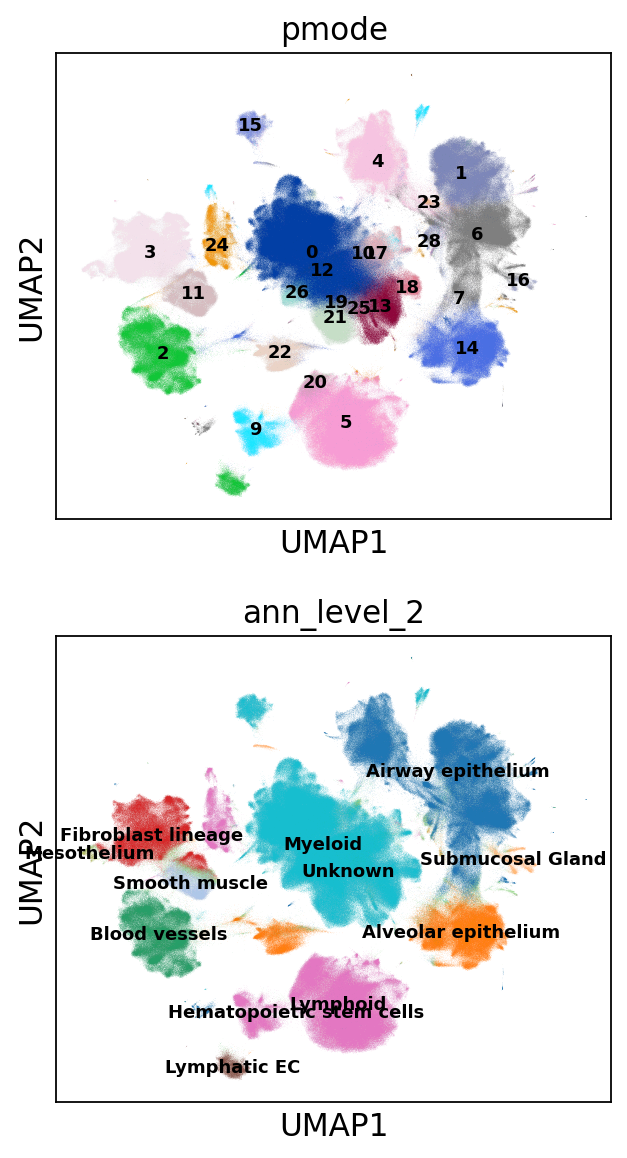
The partitions seem to grasp some clustering closely related to the original level 2 annotation.
print(skmt.adjusted_rand_score(_adata.obs['pmode'], _adata.obs['ann_level_2']))
0.5801220132920343
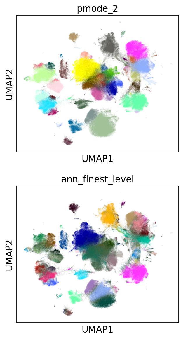
The resolution of the model depends on the subsampling ratio. We try the same procedure taking 5 times more cells
n_iter = 20
N = 10000
ski = np.zeros((n_iter, N))
X = np.arange(adata.shape[0], dtype=np.int32)
for x in range(n_iter):
    np.random.shuffle(X)
    ski[x] = X[:N]
ski = ski.astype(int)

n_obs = N
sketch_data = ad.AnnData(ssp.csr_matrix((n_obs, n_var)))
pred_labels = np.zeros((adata.shape[0], n_iter)).astype(int)
for x in tqdm(range(n_iter)):
    sketch_data.obsm[use_rep] = adata[ski[x]].obsm[use_rep].copy()
    sc.pp.neighbors(sketch_data, n_neighbors=n_neighbors, use_rep=use_rep)
    scs.inference.fit_model(sketch_data, model='ppbm')
    index = NNDescent(sketch_data.obsm['X_scanvi_emb'], n_neighbors=n_neighbors, metric='cosine', )
    C = np.array(sketch_data.obs['ppbm'].values).astype(int)
    pred = np.unique(C[index.query(query, k=5)[0]], axis=1)[:, 0]
    pred_labels[:, x] = pred

pmode = gt.PartitionModeState(pred_labels.T,
                             converge=True)
bs = pmode.get_max(g)
_adata.obs['pmode_2'] = pd.Categorical(values=np.array(bs.get_array()).astype('U'))
100%|██████████| 20/20 [1:27:19<00:00, 261.95s/it]
As expected, the time required for each loop increases. Ideally one should find a good balance between the subsampling, the number of iterations and the overall time. Comparing the partitions of the two strategies with the original extracted from the whole dataset, we notice that completeness increases in the second experiment, while homogeneity remains unchanged. This is in line with the expected behaviour as we obtain finer descriptions.
print(skmt.homogeneity_completeness_v_measure(_adata.obs['pmode'], _adata.obs['ppbm']))
print(skmt.homogeneity_completeness_v_measure(_adata.obs['pmode_2'], _adata.obs['ppbm']))
(0.7796964452269838, 0.37712915167813155, 0.5083674838135956)
(0.7664660005824697, 0.47533707936760183, 0.5867753366597966)
The effect of finer clustering can be appreciated comparing to the highest detail available for this dataset
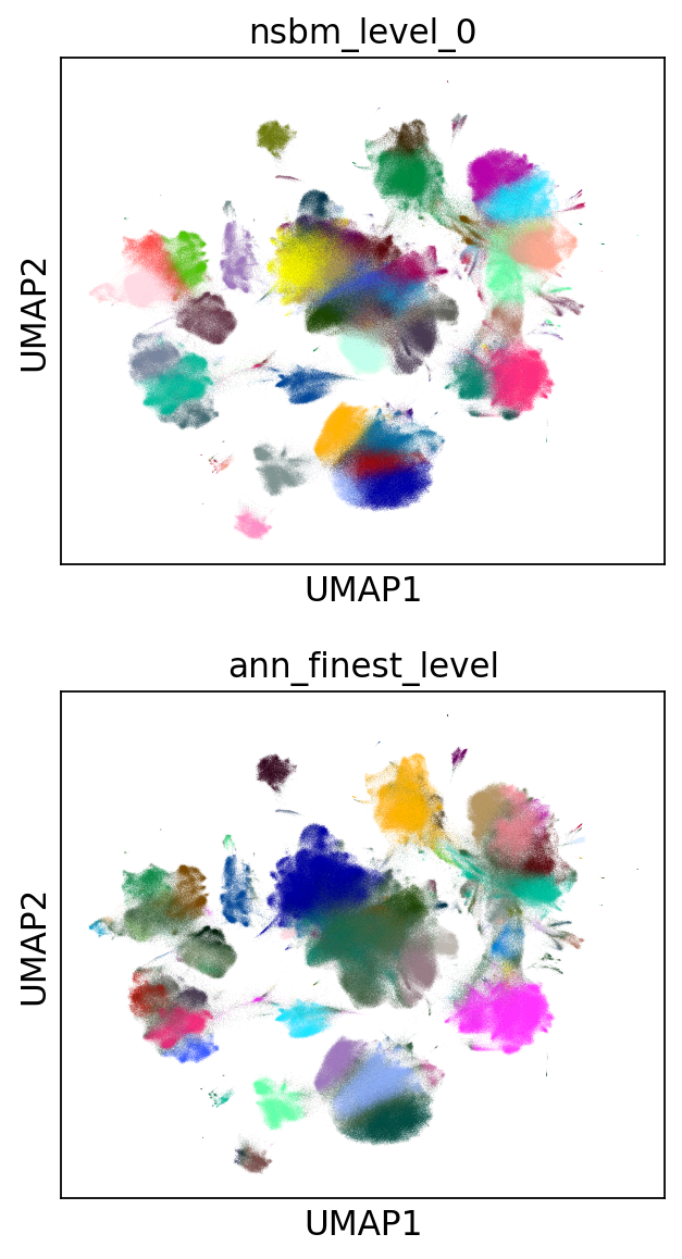
sc.pl.umap(_adata,color=['pmode_2', 'ann_finest_level'],
           ncols=1, legend_loc=None)
The default models
The ppbm is an effective approach and returns assortative
communities, in the analysis of kNN graphs derived from single cell data
it is reasonable to expect those communities to reflect the population
structure in terms of cell types. Nevertheless, we may be interested in
the Stochastic Block Model or its Nested formulation as well. Those
approach incorporate other priors in the model, possibly identifying
other properties of the dataset. While the code for the sbm
is substantially the same, for the nsbm we need to collect
the matrix of groupings at different levels. It’s sufficient to transfer
level 0 to the original dataset, the remaining levels will be mapped
using a dictionary.
n_iter = 20
N = 2000
ski = np.zeros((n_iter, N))
X = np.arange(adata.shape[0], dtype=np.int32)
for x in range(n_iter):
    np.random.shuffle(X)
    ski[x] = X[:N]
ski = ski.astype(int)

n_obs = N
sketch_data = ad.AnnData(ssp.csr_matrix((n_obs, n_var)))
pred_labels = np.zeros((adata.shape[0], n_iter)).astype(int)
for x in tqdm(range(n_iter)):
    sketch_data.obsm[use_rep] = adata[ski[x]].obsm[use_rep].copy()
    sc.pp.neighbors(sketch_data, n_neighbors=n_neighbors, use_rep=use_rep)
    scs.inference.fit_model(sketch_data, model='sbm', deg_corr=True)
    index = NNDescent(sketch_data.obsm['X_scanvi_emb'], n_neighbors=n_neighbors, metric='cosine', )
    C = np.array(sketch_data.obs['sbm'].values).astype(int)
    pred = np.unique(C[index.query(query, k=5)[0]], axis=1)[:, 0]
    pred_labels[:, x] = pred

pmode = gt.PartitionModeState(pred_labels.T,
                             converge=True)
bs = pmode.get_max(g)
_adata.obs['sbm'] = pd.Categorical(values=np.array(bs.get_array()).astype('U'))
100%|██████████| 20/20 [16:50<00:00, 50.51s/it]
The resolution for the sbm using a small subsample is similar
to the one obtained with the ppbm on larger sampling.
sc.pl.umap(_adata,color=['sbm', 'ann_finest_level'],
           ncols=1,
           legend_loc=None)
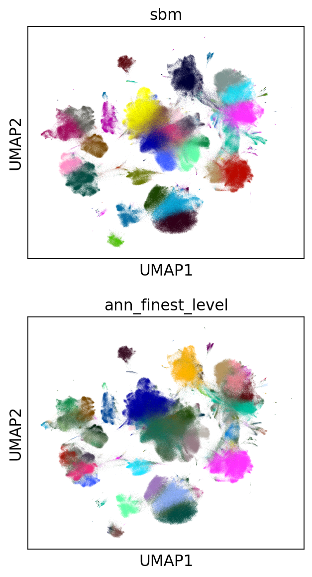
skmt.adjusted_mutual_info_score(_adata.obs['ann_finest_level'], _adata.obs['sbm'])
0.6371068117249558
Lastly we can try the nsbm
n_iter = 20
N = 2000
ski = np.zeros((n_iter, N))
X = np.arange(adata.shape[0], dtype=np.int32)

for x in range(n_iter):
    np.random.shuffle(X)
    ski[x] = X[:N]

ski = ski.astype(int)

sketch_collect = []
n_obs=N
n_neighbors=10
use_rep='X_scanvi_emb'
sketch_data = ad.AnnData(ssp.csr_matrix((n_obs, n_var)))
labels = []
for x in tqdm(range(n_iter)):
    sketch_data.obsm[use_rep] = adata[ski[x]].obsm[use_rep].copy()
    sc.pp.neighbors(sketch_data, n_neighbors=n_neighbors, use_rep=use_rep)
    scs.inference.fit_model(sketch_data)
    index = NNDescent(sketch_data.obsm['X_scanvi_emb'], n_neighbors=n_neighbors, metric='cosine', )
    C = np.array(sketch_data.obs['nsbm_level_0'].values).astype(int)
    pred0 = np.unique(C[index.query(query, k=5)[0]], axis=1)[:, 0]

    n_blocks = len(sketch_data.uns['schist']['nsbm']['blocks'])
    _label = np.zeros((adata.shape[0], n_blocks)).astype(int)
    _label[:, 0] = pred0.astype(int)
    for y in range(1, n_blocks):
        dd = dict(sketch_data.obs[[f'nsbm_level_0', f'nsbm_level_{y}']].drop_duplicates().astype(int).values)
        _label[:, y] = [int(dd[v]) for v in pred0]

    labels.append(_label)
100%|██████████| 20/20 [24:47<00:00, 74.38s/it]
In terms of computation time, we notice that nsbm >
sbm > ppbm. To proceed, we need a different way
to treat the consesus partition. First we need to create the necessary
block states.
%%time
states = []
for x in range(n_iter):
    states.append(gt.NestedBlockState(g,
                    bs=labels[x].T,
                   deg_corr=True))
CPU times: user 3min 45s, sys: 3.14 s, total: 3min 48s
Wall time: 3min 17s
%%time
pmode_nested = gt.PartitionModeState([x.get_bs() for x in states], converge=True, nested=True)
bs = pmode_nested.get_max_nested()
CPU times: user 11min 35s, sys: 616 ms, total: 11min 35s
Wall time: 11min 35s
#these lines are only needed to prune redundant top hierarchies having only one group
bs = [x for x in bs if len(np.unique(x)) > 1]
bs.append(np.array([0], dtype=np.int32)) #in case of type changes, check this
Lastly get the final block state and add all the annotations to the “empty” data
state = gt.NestedBlockState(g, bs=bs,
                            deg_corr=True)
_adata.obs['nsbm_level_0'] = bs[0].astype(str)
for x in range(1, len(state.levels)):
    _adata.obs[f'nsbm_level_{x}'] = np.array(state.project_partition(x, 0).a).astype(str)
It is worth noting that the lowest level of the hierarchy reflects the groups in a subsampled datasets, hence it won’t ever be a faithful representation of what’s in the whole dataset. It is also true that lowest levels are rarely used in the analysis, as most of the interesting cell groups appear at higher levels. Also, if this dataset contained a very rare cell population (say, less than 100 cells) it is very unlikely that it will pop out using this approach
sc.pl.umap(_adata,color=['nsbm_level_0', 'ann_finest_level'],
           ncols=1,
           legend_loc=None)
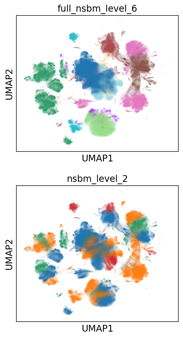
Since the NSBM includes a hierarchy, it is important to assess if the
reconstructed one is meaningful. To answer this question we need the
results of a nsbm on the whole dataset. Similarly to what
has been done with the PPBM, we externally minimized a model for that.
By comparing two highest levels of the relative hierarchies we already
appreciate how the reconstruction of the hierarchy in the subsampled
approach fails, mixing cell groups that do not belong together. Hence,
we currently discourage inference on subsampled data for the
nsbm, whereas it may be a valid approach for the remaining
models.
full_nsbm_state = pickle.load(open("HCA_full_it_1151.pickle", 'rb'))
scs._utils.plug_state(_adata, full_nsbm_state, key_added='full_nsbm')
sc.pl.umap(_adata, color=['full_nsbm_level_6', 'nsbm_level_2'], ncols=1, legend_loc=None)
Model Refinement
Since these solutions are all approximations, it may be worth to refine them, forcing a fixed number of MCMC iterations and assuming the current approximated solution would be the start of a better chain. We will run a very small number of iterations (10), in reality it may be better to increase it, depending on the available time.
ppbm_state = gt.PPBlockState(g, b=np.array(_adata.obs['pmode_2'].cat.codes))
E1 = ppbm_state.entropy()
nb1 = ppbm_state.get_nonempty_B()
for n in tqdm(range(10)):
    ppbm_state.multiflip_mcmc_sweep(beta=np.inf, niter=10, c=0.5)
E2 = ppbm_state.entropy()
nb2 = ppbm_state.get_nonempty_B()
100%|██████████| 10/10 [13:13<00:00, 79.39s/it]
print(f"Entropy before refinement: {E1}")
print(f"Entropy after refinement: {E2}")
print(f"Entropy difference: {E2 - E1}")
print(f"Number of blocks before refinement: {nb1}")
print(f"Number of blocks after refinement: {nb2}")
Entropy before refinement: 487045167.6521903
Entropy after refinement: 463980334.0686416
Entropy difference: -23064833.583548725
Number of blocks before refinement: 61
Number of blocks after refinement: 76
scs._utils.plug_state(_adata, ppbm_state, key_added='refined_ppbm')
if nb2 > 100:
    _adata.uns['refined_ppbm_colors'] = [mpl.colors.rgb2hex(x) for x in cm.gist_ncar(np.linspace(0, 1, nb2))]
sc.pl.umap(_adata, color='refined_ppbm', legend_loc=None)
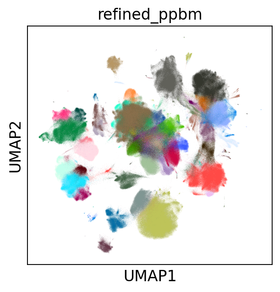
Of course, the refinement has a minimal impact in this example, as we
ran only 10 iterations. Refinement could be a solution to correctly reconstruct the hierarchy of the nsbm, although the time spent on this may defeat the approach of subsampling.
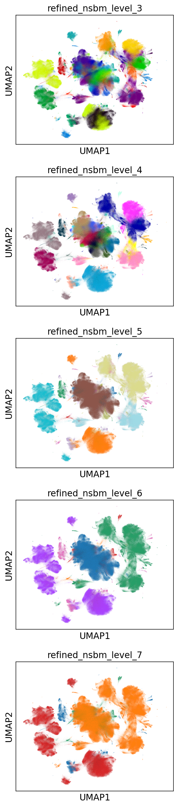
bs = pmode_nested.get_max_nested()
nsbm_state = gt.NestedBlockState(g, bs=bs,
                            deg_corr=True)
E1 = nsbm_state.entropy()
nb1 = nsbm_state.get_levels()[0].get_nonempty_B()
for n in tqdm(range(500)):
    nsbm_state.multiflip_mcmc_sweep(beta=np.inf, niter=10, c=0.5)
E2 = nsbm_state.entropy()
nb2 = nsbm_state.get_levels()[0].get_nonempty_B()
100%|██████████| 500/500 [25:25:03<00:00, 183.01s/it]
print(f"Entropy before refinement: {E1}")
print(f"Entropy after refinement: {E2}")
print(f"Entropy difference: {E2 - E1}")
print(f"Number of blocks before refinement (level 0): {nb1}")
print(f"Number of blocks after refinement (level 0): {nb2}")
Entropy before refinement: 468677546.2346465
Entropy after refinement: 326768701.60364324
Entropy difference: -141908844.63100326
Number of blocks before refinement (level 0): 60
Number of blocks after refinement (level 0): 4210
After refinement the hierarchy looks more consistent, although it took almost one day to compute.
scs._utils.plug_state(_adata, nsbm_state, key_added='refined_nsbm')
for level in range(3, 8):
    nb2 = len(_adata.obs[f'refined_nsbm_level_{level}'].cat.categories)
    if nb2 > 100:
        _adata.uns[f'refined_nsbm_level_{level}_colors'] = [mpl.colors.rgb2hex(x) for x in cm.nipy_spectral(np.linspace(0, 1, nb2))]
to_plot = [f'refined_nsbm_level_{level}' for level in range(3, 8)]
sc.pl.umap(_adata, color=to_plot, legend_loc=None, ncols=1)
Conclusions
How do these solutions compare to a model that takes the whole dataset?
For the ppbm and the sbm the subsampled
solutions can be considered coarser descriptions of the same model computed on the entire dataset. In the full model, the partition sizes are rather small compared to the
size of the dataset. The full sbm, in particular, will find thousands of groups (given that \(B \propto \sqrt{N}\), we may expect 103 groups in this case), which may be unpractical to analyze. Since the model from subsampled data will raise many less groups, the subsampled solution may even be preferable. As for the nsbm, we will obtain a even coarser description compared to the same model on the entire dataset; the nested model, in fact, is able to identify smaller groups (\(B \propto N\log(N)\), 105 in this case). In addition, we should ensure that the hierarchy is somehow consistent, otherwise we should drop (for now) the possibility to subsample data for the nsbm, unless some time is spent on model refinement.