Clustering of 3k PBMCs
In this section, the “3k PBMCs” dataset is preprocessed, using scanpy. Afterwards, cluster analysis is performed, using schist.
The first step necessary to perform cluster analyses with schist is to import the library:
import schist as scs
After that, standard analysis with scanpy can be performed:
import scanpy as sc

adata=sc.read(adata = sc.read_10x_mtx('data/filtered_gene_bc_matrices/hg19/', var_names='gene_symbols', cache=True)
sc.pp.filter_cells(adata, min_genes=200)
sc.pp.filter_genes(adata, min_cells=3)
mito_genes = adata.var_names.str.startswith('MT-')
adata.obs['percent_mito'] = np.sum(adata[:, mito_genes].X, axis=1) / np.sum(adata.X, axis=1)
adata.obs['n_counts'] = adata.X.sum(axis=1)
adata = adata[adata.obs['percent_mito'] < 0.05, :]
sc.pp.normalize_total(adata, target_sum=1e4)
sc.pp.log1p(adata)
sc.pp.highly_variable_genes(adata, min_mean=0.05, max_mean=3, min_disp=0.5)
adata = adata[:, adata.var.highly_variable]
sc.pp.regress_out(adata, ['n_counts', 'percent_mito'])
sc.pp.scale(adata, max_value=10)
sc.tl.pca(adata)
Before the cluster analysis with schist, the k-NN graph must be built, representing connections between cells of the dataset. The k-NN graph can be created, using the scanpy function sc.pp.neighbors(), which allows the selection of the number of neighbors and the number of pca components considered for the analysis:
sc.pp.neighbors(adata, n_neighbors=20, n_pcs=30)
Moreover, in order to spatially visualize the outcome of cluster analysis, we can compute the UMAP embedding of our dataset, using the function sc.tl.umap():
sc.tl.umap(adata)
Nested Model
The most prominent function implemented in schist library is the clustering function schist.inference.fit_model(). It relies on a process called minimization of the description length, implemented in the graph-tool python library:
in lay terms, different partitions representig the dataset are generated;
after that, the partition with the lowest description length is selected as the final output (the simplest partition among partitions with the highest explanatory power).
However, the minimization of the description length could fall into local minima. Therefore, another approach has been implemented in graph-tool:
in particular, the minimization step can be called multiple times;
the partition with the lowest description lenght is stored for each round of minimization;
finally, each stored partition is explored, in order to build a single partition, which considers each minimum.
Pratically, this can be achieved, using schist:
scs.inference.fit_model(adata, n_init=100)
The parameter n_init accounts for the number of minimization step performed: the larger the number of rounds, the slower the process. n_init parameter is set at 100 by default.
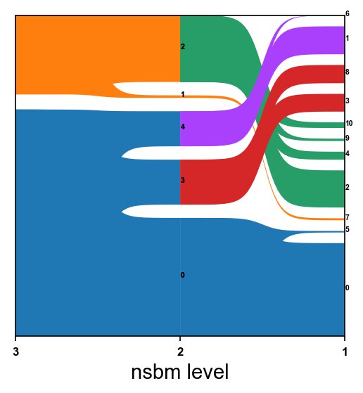
In order to effectively visualize the nested hierarchy representing the partition, we have implemented the function schist.plotting.alluvial():
scs.plotting.alluvial(adata)

The hierarchy can be furtherly cut, using the parameters level_start and level_end:
scs.plotting.alluvial(adata, level_start=1, level_end=3)
The final outcome of the function schist.inference.fit_model() consists of a series of nested levels, stored in adata.obs, with the prefix nsbm_level_ followed by a number, expressing the level of the hierarchy. Each level can be visualized thanks to the scanpy function sc.pl.umap():
sc.pl.umap(adata, color=['nsbm_level_0', 'nsbm_level_1', 'nsbm_level_2', 'nsbm_level_3', 'nsbm_level_4'], ncols=2, legend_loc='on data')

Planted Model
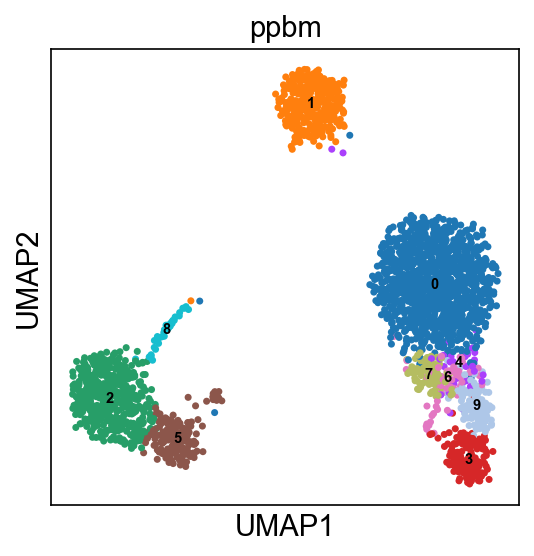
The nested model is expected to find reliable communities in networks, however, it pays its statistical significance in terms of runtimes. Another approach implemented in graph-tool, called Planted Partition Block Model, performs Bayesian inference on node groups. This function, in particular, uses the Planted Block Model, which is particularly suitable in case of assortative graphs and it returns the optimal number of communities:
scs.inference.fit_model(adata, model='ppbm')
The final outcome of the function consists of a single layer of annotations, stored in adata.obs, with the prefix ppbm, which can be visualized through sc.pl.umap():
sc.pl.umap(adata, color=['ppbm'], legend_loc='on data')