Combined analysis of multimodal DBiT-seq data

In this page we show how to perform multimodal integration of spatially resolved data. We previously performed ATAC and RNA analysis. We start loading required libaries and load the previously saved data.

import numpy as np
import pandas as pd
import matplotlib
import matplotlib.pyplot as plt
from matplotlib.pyplot import *

import anndata as ad
import scanpy as sc
import scipy.sparse as ssp

import spatialdata_io
import spatialdata_plot
import spatialdata as sd

import squidpy as sq
import schist as scs
import warnings
warnings.filterwarnings('ignore')

def set_res(high=True):
        dpi=80
        if high:
                dpi=150
        sc.set_figure_params(dpi=dpi, fontsize=6)
        rcParams['axes.grid'] = False

set_res(False)

Here we actually load data

atac = sd.read_zarr('analysis/SRR22565186.zarr')
rna = sd.read_zarr('analysis/SRR22561636.zarr')

We here perform the analysis without the need of having the same pixels in both datasets. That means we need a single spatial graph that is the union of RNA and ATAC, yet we have to keep it ordered, to recreate the proper spatial coordinates.

all_cells = atac.table.obs_names.union(rna.table.obs_names)
emx = ssp.csr_matrix((len(all_cells), 1), dtype=np.int32)

_tmp =ad.AnnData(emx)
_tmp.obs_names = all_cells
_tmp.obs[['array_A', 'array_B']] = 0
for coord in ['array_A', 'array_B']:
        _tmp.obs[coord] = rna.table.obs[coord]
        for p in atac.table.obs_names:
                _tmp.obs[coord][p] = atac.table.obs[coord][p]

idx = _tmp.obs.sort_values(by=["array_A", "array_B"]).index
_tmp = _tmp[idx]
_tmp.obsm['spatial'] = _tmp.obs[['array_A', 'array_B']].values
_tmp.obs["pixel_id"] = np.arange(len(_tmp.obs_names))

On the temporary dataset (_tmp) we compute the spatial graph using squidpy

sq.gr.spatial_neighbors(_tmp, n_neighs=8, coord_type='grid')

Now we can all the nested model on three modalities (actually 2 + spatial) to get the final results. The three dataset share pixel names, which allows proper alignment. Yet, RNA and ATAC do not have all pixels in common.

sc.settings.verbosity=2
scs.inference.fit_model_multi([atac.table, rna.table, _tmp], key_added='mspt',
                              neighbors_key=['spectral_neighbors', 'pca_neighbors',
                              'spatial_neighbors'])
sc.settings.verbosity=0

minimizing the nested Stochastic Block Model
getting adjacency for data 0 (0:00:00)
getting adjacency for data 1 (0:00:00)
getting adjacency for data 2 (0:00:00)
        minimization step done (0:10:57)
        consensus step done (0:11:15)
    done (0:11:15)
    finished (0:11:15)

The clusters will be the same for RNA and ATAC, even if the set of pixels does not overlap completely. From this point on, one can proceed calling differential features across structures or, for example, performing spatial trajectory analysis incorporating from two modalities. First, here’s the result for RNA

set_res(True)
rna.pl.render_images().pl.render_shapes(color='mspt_level_1', fill_alpha=.7).pl.show(title='SPT_level_1', colorbar=True)
xticks([])
yticks([])
plt.xlabel('A barcodes')
plt.ylabel('B barcodes')

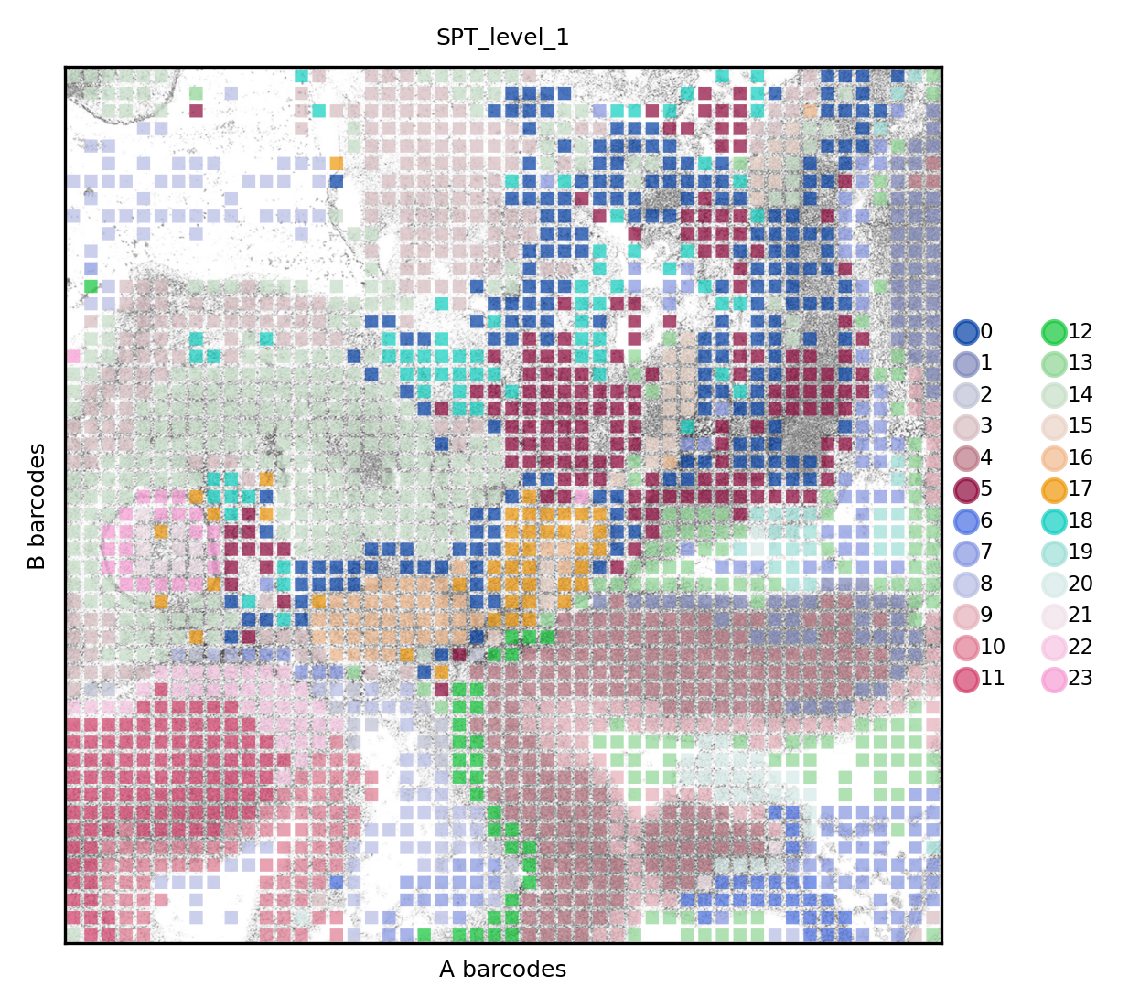
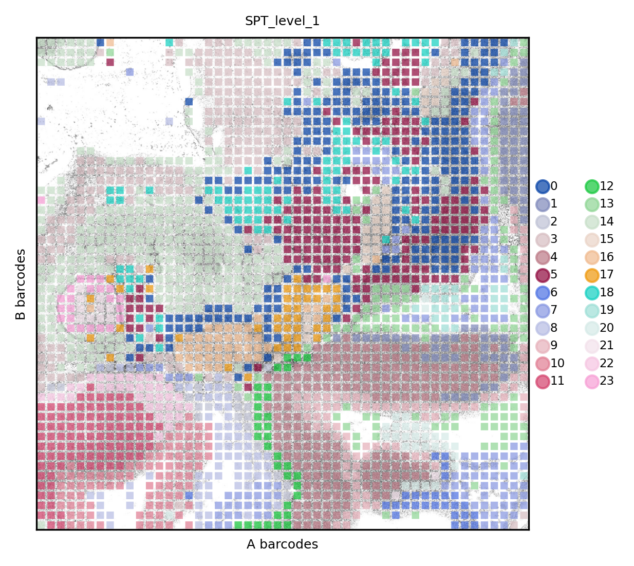
And the result for ATAC

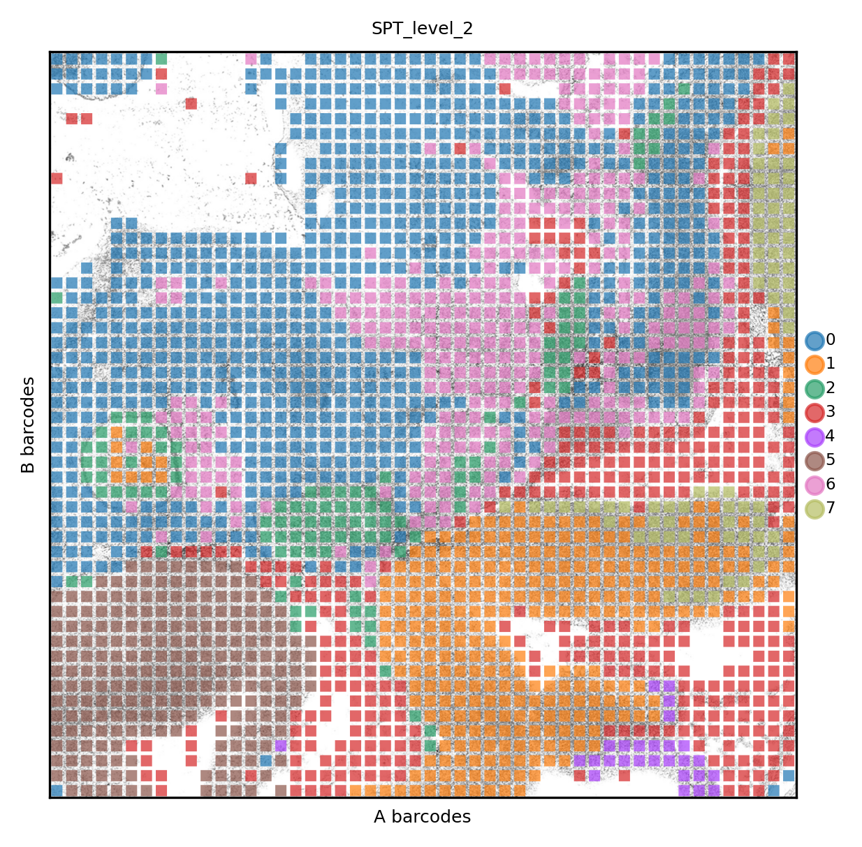
The same data can be visualized at a coarser resolution (level 2)

set_res(True)
atac.pl.render_images().pl.render_shapes(color='mspt_level_2', fill_alpha=.7).pl.show(title='SPT_level_2', colorbar=True)
xticks([])
yticks([])
plt.xlabel('A barcodes')
plt.ylabel('B barcodes')

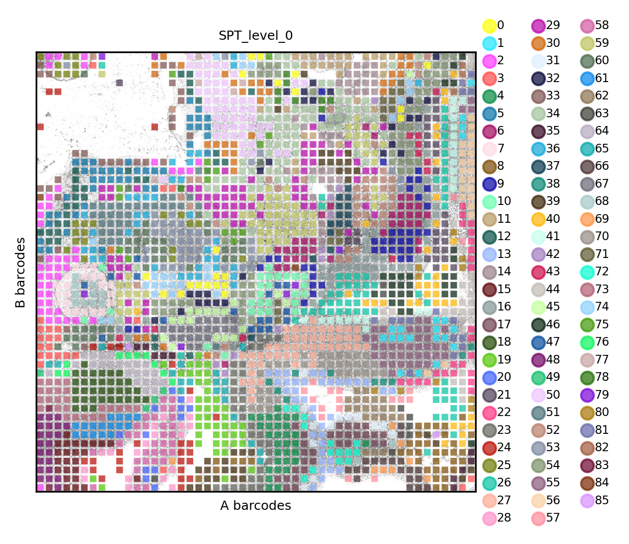
Or higher (level 0), which represent the finest, statistically supported, description of this dataset.