Analysis of spatially resolved RNA-seq data
Similarly to what shown analyzing ATAC data, we retrieved fastq from the paper “Spatial epigenome–transcriptome co-profiling of mammalian tissues” (Zhang et al, 2023, DOI:10.1038/s41586-023-05795-1), this time RNA sequences (SRA run ID: SRR22561636) and processed using kb_python. The resulting count matrix file is imported and processed as standard scRNA-seq data
import numpy as np
import pandas as pd
import matplotlib
import matplotlib.pyplot as plt
from matplotlib.pyplot import *

import anndata as ad
import scanpy as sc

import scipy.sparse as ssp
import scipy.stats as sst

import spatialdata_io
import spatialdata_plot
import spatialdata as sd

import squidpy as sq
import schist as scs
import warnings
warnings.filterwarnings('ignore')
#import magic
from tqdm import tqdm

def set_res(high=True):
        dpi=80
        if high:
                dpi=150
        sc.set_figure_params(dpi=dpi, fontsize=6)
        rcParams['axes.grid'] = False

set_res(False)
First we import the .h5ad file computed by kb_python. After that we perform some QC and filtering, as proposed by sc-best-practices.
adata = sc.read_h5ad("SRR22561636/counts_unfiltered/adata.h5ad")

adata.var["mt"] = adata.var_names.str.startswith("mt-")
adata.var["ribo"] = adata.var_names.str.startswith(("Rps", "Rpl"))
sc.pp.calculate_qc_metrics(
        adata, qc_vars=["mt", "ribo"], inplace=True, percent_top=[20], log1p=True
)

def is_outlier(adata, metric: str, nmads: int):
        M = adata.obs[metric]
        outlier = (M < np.median(M) - nmads * sst.median_abs_deviation(M)) | (
                np.median(M) + nmads * sst.median_abs_deviation(M) < M
        )
        return outlier

adata.obs["outlier"] = (
        is_outlier(adata, "log1p_total_counts", 5)
        | is_outlier(adata, "log1p_n_genes_by_counts", 5)
        | is_outlier(adata, "pct_counts_in_top_20_genes", 5)
)


adata.obs["mt_outlier"] = is_outlier(adata, "pct_counts_mt", 3) | (
        adata.obs["pct_counts_mt"] > 8
)
In the end we retain most of the pixels
print(f"Total number of cells: {adata.n_obs}")
adata = adata[(~adata.obs.outlier) & (~adata.obs.mt_outlier)].copy()
print(f"Number of cells after filtering of low quality cells: {adata.n_obs}")
Total number of cells: 2500
Number of cells after filtering of low quality cells: 2157
We select highly variable genes and then perform normalization (PFlog1pPF). Lastly, after PCA is computed, we save the anndata to build later the spatialdata object.
sc.pp.highly_variable_genes(adata,  flavor='seurat_v3_paper')

pf = adata.X.sum(axis=1).A.ravel()
l1pf = np.log1p(ssp.diags(pf.mean()/pf)@adata.X)
pf = l1pf.sum(axis=1).A.ravel()
adata.X = ssp.diags(pf.mean()/pf)@l1pf

sc.tl.pca(adata, use_highly_variable=True)
adata.write("analysis_rna/rna.h5ad")
Here the anndata is imported using the DBiT-seq plugin for spatialdata. Note that we had to rotate the original image from the paper 90 degrees CCW, as the current version of the plugin orders the barcodes differently from what is displayed in the original paper.
spdata = spatialdata_io.readers.dbit.dbit(path='analysis_rna',
                                     anndata_path='analysis_rna/rna.h5ad',
                                     barcode_position='barcodes.txt',
                                     image_path='ME13_50um_spatial/tissue_hires_image.png',
                                     dataset_id='ME13_50um_spatial')
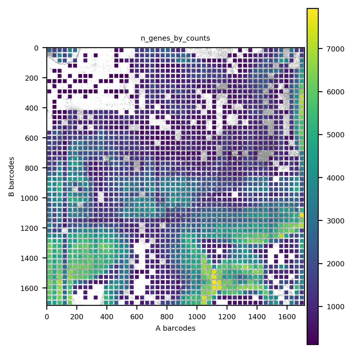
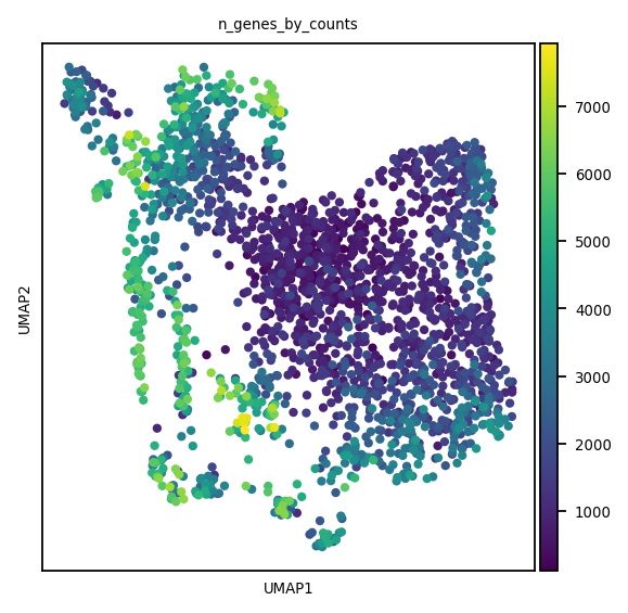
We can visualize a QC value (number of genes) in its context
We create the kNN graph using the PCA embedding, then we apply schist to find the hierarchical cell structure
basis='pca'
sc.settings.verbosity=2
scs.inference.fit_model(spdata.table,
                                                   neighbors_key=f'{basis}_neighbors')
sc.settings.verbosity=0
minimizing the nested Stochastic Block Model
        minimization step done (0:01:14)
        consensus step done (0:01:25)
    done (0:01:25)
    finished (0:01:25)
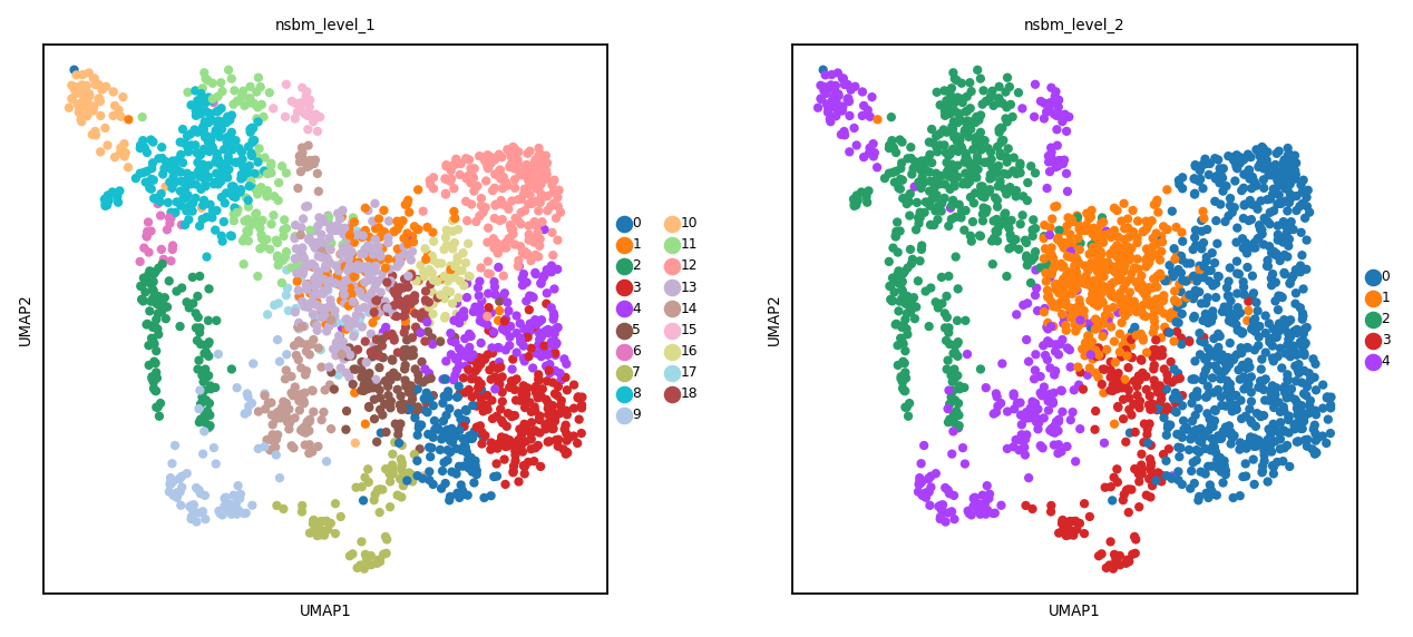
sc.pl.umap(spdata.table, color=['nsbm_level_1', 'nsbm_level_2'])
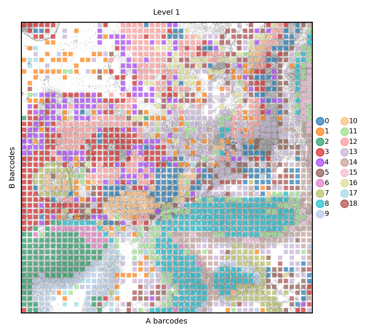
Finally we can check how clusters distribute in their spatial context. At level 1 we can distinguish certain clusters that belong to the neual tissues. Here the results appear to be in line with the publication
set_res(True)
spdata.pl.render_images().pl.render_shapes(color='nsbm_level_1', fill_alpha=.7).pl.show(title='Level 1', colorbar=True)
xticks([])
yticks([])
plt.xlabel('A barcodes')
plt.ylabel('B barcodes')
Similarly to what has been done for ATAC, we perform the analysis of a multimodal data, where one modality is represented by the spatial graph
sq.gr.spatial_neighbors(spdata.table, n_neighs=8, coord_type='grid')

_tmp = spdata.table.copy()
sc.settings.verbosity=2
scs.inference.fit_model_multi([spdata.table, _tmp],
                              key_added='spt',
                              neighbors_key=['pca_neighbors', 'spatial_neighbors'])
sc.settings.verbosity=0
minimizing the nested Stochastic Block Model
getting adjacency for data 0 (0:00:00)
getting adjacency for data 1 (0:00:00)
        minimization step done (0:04:11)
        consensus step done (0:04:21)
    done (0:04:21)
    finished (0:04:22)
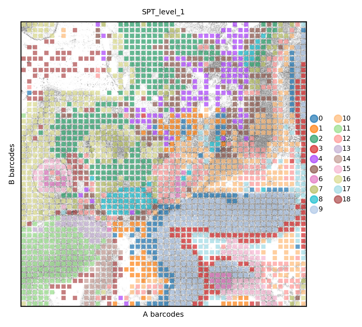
Again, we visualize the structured data, with a better resolution of anatomical structures
set_res(True)
spdata.pl.render_images().pl.render_shapes(color='spt_level_1', fill_alpha=.7).pl.show(title='SPT_level_1', colorbar=True)
xticks([])
yticks([])
plt.xlabel('A barcodes')
plt.ylabel('B barcodes')
Again, we save data for later use in integrated analysis.
spdata.write('analysis/SRR22561636.zarr')